Aggregation & Downsampling
By default a widget receives raw rows: every record that matches its filters, newest first, up to the row limit. That is exactly right for a table of the latest readings, and exactly wrong for a chart of the last six months — a sensor sampling every second produces 15 million rows in that window, of which a 600-pixel-wide chart can draw perhaps 600.
Aggregation solves both problems at once. The project database groups the matching records into time buckets, computes one value per bucket, and sends only those values to the widget. A year of data becomes a few hundred points, and questions the raw data cannot answer — average temperature per hour, records per machine, total energy today — become ordinary widget configuration.
Everything happens in the database, before the data reaches the browser. Nothing is computed in the widget, so aggregated widgets stay live and stay fast regardless of how much history sits behind them.
Turning It On
Aggregation lives in the same dialog as filters — the one that opens from the filter icon next to a data binding. See Data Binding for the dialog as a whole.
Inside, the Aggregation section offers two choices:
- Raw rows — the default: records are returned as they are stored.
- Aggregated over time — records are grouped and reduced to one value per group.
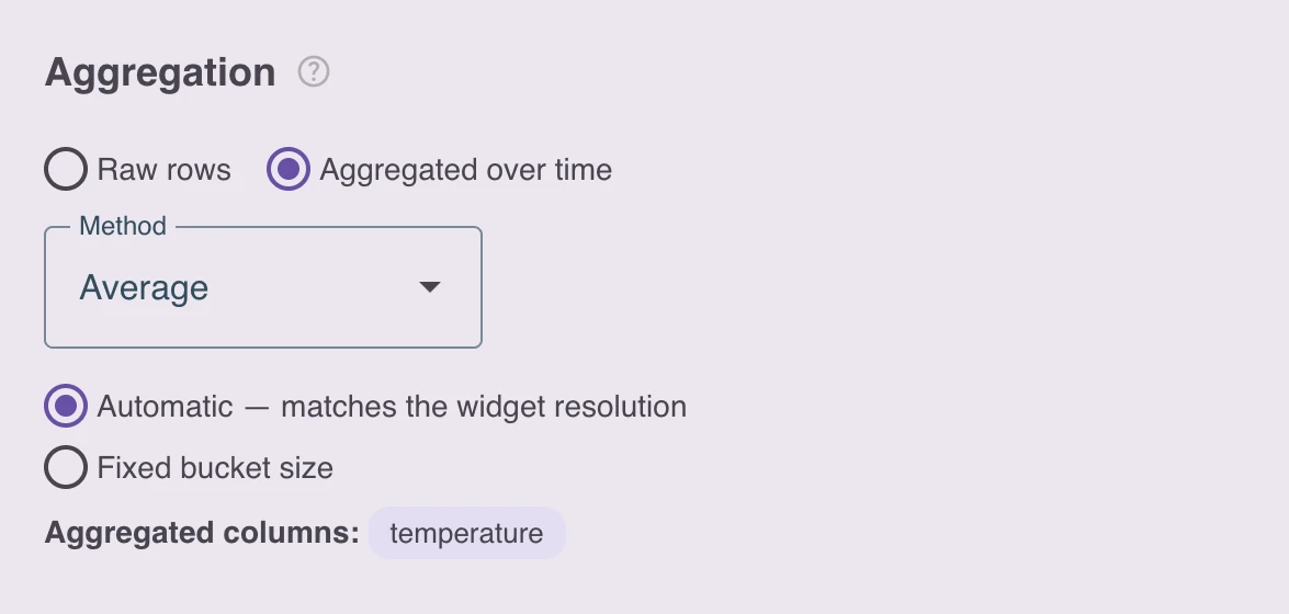
Switching to Aggregated over time reveals a Method selector and, where applicable, the bucket-size controls described below. Because every aggregate needs a time range to work on, enabling aggregation also fills in a default rolling window of the last 24 hours if the widget did not have a time window yet — adjust it in the Rolling time window section directly above.
Methods
| Method | Result per bucket | Works on |
|---|---|---|
| Average | Arithmetic mean of the values | Numeric columns |
| Sum | Total of the values | Numeric columns |
| Count | Number of records with a value | Any column |
| Minimum | Smallest value | Numeric, text and timestamp columns |
| Maximum | Largest value | Any of the above |
| First value | Value of the earliest record in the bucket | Any column |
| Last value | Value of the latest record in the bucket | Any column |
One method applies to all value columns of a single data series. To show several statistics of the same measurement — a minimum/maximum band with an average line, for example — add one data series per statistic. They share a single database query, so the extra series cost nothing in requests.
Average, Sum, Minimum and Maximum require a column that holds numbers. Pointing them at a text or boolean column is rejected with an explanatory message. Count works on anything, which makes it the method for “how many records” questions.
What Gets Aggregated
You never list columns for the aggregation explicitly — the platform derives them from the field mapping you already configured for the widget:
| Field role | Meaning under aggregation |
|---|---|
x = tsp | The chart has a time axis: buckets subdivide the time window. |
| x = any other column | The chart has a category axis: that column groups the records. |
| pivot | Splits the result into one series per distinct value, aggregated separately. |
| y, r, and other value fields | Aggregated with the selected method. |
This means the same mapping you use for raw rows keeps working: map x to the timestamp and y to temperature, switch on aggregation, and the chart plots average temperature per bucket instead of every individual reading.
The Three Shapes of an Aggregated Widget
1. Time series with automatic resolution
The most common case: x is mapped to tsp and the bucket mode is left on Automatic — matches the widget resolution. The platform then picks the bucket size from the widget’s rendered width — a chart that is 600 pixels wide never receives more than about 600 points, whatever the time window. Widen the window from a day to a year and the buckets simply get wider; the amount of data crossing the network stays constant.
Choose this when the bucket size itself carries no meaning and you only want a readable, fast chart of a trend: “temperature over the last month”.
Resizing a widget re-fetches at the new resolution, but only when the width crosses a step — small drags do not trigger requests.
2. Time series with a fixed bucket size
Select Fixed bucket size and specify a length and a unit — every 1 hour, every 15 minutes, every 6 hours. Use this whenever the interval is part of the question rather than a display detail: “units produced per hour”, “energy consumed per day”.
Fixed buckets are aligned to natural boundaries in your browser’s time zone: 6-hour buckets start at 00:00, 06:00, 12:00 and 18:00 local time; daily buckets break at local midnight; weekly buckets start on Monday.
If the chosen size would produce more buckets than a chart can sensibly show (the cap is 2000), the platform automatically widens the buckets to a multiple of what you asked for — one-minute buckets over a full week become five-minute buckets — rather than refusing the query. The dialog tells you when this happens and which size is actually used.
3. One value per category
Map x to a column instead of the timestamp — a machine name, a product type, a site — and the widget becomes a categorical summary: the entire time window is treated as a single bucket, and every distinct value of that column yields exactly one aggregated row.
This is the shape for “records per machine today” or “average cycle time per production line this week”. There is no bucket size to choose — the dialog says so instead of showing the interval controls.
Counting records: the row count of a group is Count applied to the timestamp column tsp, since every record has one. Map y to tsp, and the platform selects Count automatically — it is the only aggregate a timestamp column allows.
x     → machine_name        (groups the records)
y     → tsp                 (counted → number of records)
Method: Count
Window: last 1 day
The result is one bar per machine showing how many records that machine produced in the last day.
Aggregated Single Values
Scalar bindings — the value of a KPI tile, a gauge, a text field — offer the same choice under a Value section:
- Latest value — the newest record’s value, as before.
- Aggregated over a time window — one value computed over the whole window.
Use it for live headline numbers: “units produced today” (Count over tsp with a 1-day window), “average temperature this shift”, “peak power this month”. There is no bucket size here either — the window is the bucket. The value refreshes as new records arrive, so unlike a number pasted into the widget it never goes stale.
Filters, Windows and Aggregation Together
The dialog’s sections apply in the order they are shown, which is also the order the database applies them:
- Rolling time window / custom time range — selects the period.
- Filters — select which records within that period participate.
- Aggregation — reduces the selected records to one value per bucket.
- Row limit — a backstop, see below.
Because filters run before aggregation, they narrow what goes into each bucket. machine = 'A' combined with hourly averages gives the hourly average for machine A. Filters bound to filter widgets or routing segments work exactly as they do for raw rows, so an aggregated chart follows a dropdown or a page URL like any other widget.
Calendar widgets compose too: when the user picks a date range, that range replaces the rolling window and the aggregation follows it.
Window snapping
While aggregation is active, the start of the window snaps to the bucket grid so the buckets themselves stay put as time passes — without it, every refresh would shift all bucket boundaries slightly and the whole chart would shimmer. The dialog notes this with “Window shifts in … steps.”, and the resolved start/end preview always shows the range actually queried.
The end of the window is never extended: a window ending now keeps ending now, and a window ending an hour ago never reaches into that last hour.
The row limit under aggregation
The Row limit stays visible but changes role: the number of buckets is derived from the widget size or from your fixed interval, not from this field. It applies only if a widget has to fall back to raw rows — for example on a self-hosted instance whose platform version predates aggregation. Leaving it at a sensible value keeps such a widget usable.
Gaps in the Data
A bucket in which no record matched is omitted from the result, not returned as zero. For an average this is the honest answer — there is no average of nothing — but for a Count chart of an intermittent event it means a line chart draws a straight line across the quiet period instead of dropping to zero. Bar charts show the gap naturally; for line charts, be aware of the difference between “no data” and “zero”.
Live Updates
Aggregated widgets stay live. As records arrive, the affected buckets are recomputed and the widget refreshes — at most once every few seconds, so a device publishing at high frequency cannot flood the board. Because the newest bucket is usually still filling, its value keeps changing until the bucket closes; this is expected, and it is why the last point of a live chart is often lower than its neighbours for Count and Sum.
Performance and Long Histories
Aggregation over a long window still has to read the records behind it. For tables that routinely back long-window charts, an app can declare continuous downsampling in its data schema — see downsample in the Data Backend reference. The platform then maintains a pre-aggregated copy of the table and answers long-window queries from it, typically orders of magnitude faster, and can retain that downsampled history longer than the raw data itself — so a chart can still show two years of hourly averages after the raw records have been dropped.
This is entirely transparent to the board: the widget configuration does not change, and queries that the pre-aggregated copy cannot serve (very fine intervals, filters on columns it does not group by) fall back to the raw table automatically.
Limitations
- Aggregation applies to tables, not to transform tables. Aggregate the underlying table instead, or pre-aggregate in the transform’s own SQL — saving a custom transform is how you do that yourself, without changing the app. It is also the way to build a widget on something aggregation cannot express at all, such as a ratio of two columns or a figure joined across two apps.
- One method per data series. Use several data series for several statistics of one column.
- Timestamps are aggregated only by Count.
Averageof a timestamp is not meaningful and is rejected. - A category axis and a time axis are mutually exclusive for one data series — a chart is either “over time” or “per category”. To get both (per-machine hourly averages), keep
xontspand put the machine column in pivot. - JSON fields can be aggregated like ordinary columns, but only fields the app declared for downsampling benefit from the pre-aggregated copy; others are computed from the raw table.
Recipes
| You want | x | y | Method | Interval |
|---|---|---|---|---|
| Temperature trend over a month | tsp | temperature | Average | Automatic |
| Units produced per hour | tsp | tsp | Count | Fixed, 1 hour |
| Energy consumed per day | tsp | kwh | Sum | Fixed, 1 day |
| Peak power per hour, per machine | tsp | power (+ pivot machine) | Maximum | Fixed, 1 hour |
| Records per machine today | machine | tsp | Count | — (category) |
| Average cycle time per line this week | line | cycle_time | Average | — (category) |
| Units produced today (KPI tile) | — | tsp | Count | — (single value) |
Summary
- Switch a binding from Raw rows to Aggregated over time in the filter dialog to have the database compute values instead of shipping records.
- With
xon the timestamp you get a time series — automatic resolution for trends, a fixed interval when the interval is the question. - With
xon another column you get one value per category; with a scalar binding you get one live number. - Count on the
tspcolumn is how you count records. - Filters apply before aggregation; empty buckets are omitted; the row limit becomes a fallback safeguard.
- For long histories, apps can declare
downsampleso the platform serves charts from a pre-aggregated copy and can keep that history beyond the raw retention window.